이 포스트는 tensorflow 1.15.0 버전을 기반으로 작성되었습니다.
해당 포스트는 Andy Bosyi의 포스트를 번역한 내용입니다. https://towardsdatascience.com/active-learning-on-mnist-saving-on-labeling-f3971994c7ba
MNIST로 Active Learning 하기
Active Learning은 학습 과정 (loss) 관점에서 가장 중요한 샘플을 선택하여 적은 데이터에 레이블을 지정할 수있는 semi-supervised 기법입니다. 데이터 양이 많고 라벨링을 해야하는 비율이 많은 경우 프로젝트 비용에 큰 영향을 줄 수 있습니다. 비율이 높습니다. 예를 들어, Object Detection 및 NLP-NER 문제가 있습니다. 이 포스트는 다음 코드를 기반으로합니다. Active Learning on MNIST
실험을 위한 데이터
# load 4000 of MNIST data for train and 400 for testing
(x_train, y_train), (x_test, y_test) = tf.keras.datasets.mnist.load_data()
x_full = x_train[:4000] / 255
y_full = y_train[:4000]
x_test = x_test[:400] /255
y_test = y_test[:400]
x_full.shape, y_full.shape, x_test.shape, y_test.shape

# 출력 값
# ((4000, 28, 28), (4000,), (400, 28, 28), (400,))
plt.imshow(x_full[3999])

레이블과 10K개 테스트 샘플이있는 60K개 숫자의 MNIST 데이터 세트를 사용합니다. 보다 빠른 훈련을 위해 훈련에 4000 개의 샘플 (사진)이 필요하고 테스트에 400 개가 필요합니다 (신경망은 훈련 중에는 이를 보지 못합니다). 정규화를 위해 그레이 스케일 이미지 포인트를 255로 나눕니다.
모델, 훈련, 라벨링 과정
# build computation graph
x = tf.placeholder(tf.float32, [None, 28, 28])
x_flat = tf.reshape(x, [-1, 28 * 28])
y_ = tf.placeholder(tf.int32, [None])
W = tf.Variable(tf.zeros([28 * 28, 10]), tf.float32)
b = tf.Variable(tf.zeros([10]), tf.float32)
y = tf.matmul(x_flat, W) + b
y_sm = tf.nn.softmax(y)
loss = tf.reduce_mean(tf.nn.sparse_softmax_cross_entropy_with_logits(labels=y_, logits=y))
train = tf.train.AdamOptimizer(0.1).minimize(loss)
accuracy = tf.reduce_mean(tf.cast(tf.equal(y_, tf.cast(tf.argmax(y, 1), tf.int32)), tf.float32))
softmax 출력 y_sm은 숫자의 확률을 나타낸다. Loss는 예측 된 데이터와 라벨링 된 데이터 사이의 전형적인 “softmax”교차 엔트로피가 될 것입니다. 유명한 Adam을 optimizer로 선택했습니다.(원문에서 유명해서 선택했다고 합니다,,) Learning rate는 기본 0.1로 설정했습니다. 위의 정확도(accuracy)를 테스트 데이터셋에서도 사용합니다.
def reset():
    '''Initialize data sets and session'''
    global x_labeled, y_labeled, x_unlabeled, y_unlabeled
    x_labeled = x_full[:0]
    y_labeled = y_full[:0]
    x_unlabeled = x_full
    y_unlabeled = y_full
    tf.global_variables_initializer().run()
    tf.local_variables_initializer().run()

def fit():
    '''Train current labeled dataset until overfit.'''
    trial_count = 10
    acc = sess.run(accuracy, feed_dict={x:x_test, y_:y_test})
    weights = sess.run([W, b])
    while trial_count > 0:
        sess.run(train, feed_dict={x:x_labeled, y_:y_labeled})
        acc_new = sess.run(accuracy, feed_dict={x:x_test, y_:y_test})
        if acc_new <= acc:
            trial_count -= 1
        else:
            trial_count = 10
            weights = sess.run([W, b])
            acc = acc_new

    sess.run([W.assign(weights[0]), b.assign(weights[1])])
    acc = sess.run(accuracy, feed_dict={x:x_test, y_:y_test})
    print('Labels:', x_labeled.shape[0], '\tAccuracy:', acc)

def label_manually(n):
    '''Human powered labeling (actually copying from the prelabeled MNIST dataset).'''
    global x_labeled, y_labeled, x_unlabeled, y_unlabeled
    x_labeled = np.concatenate([x_labeled, x_unlabeled[:n]])
    y_labeled = np.concatenate([y_labeled, y_unlabeled[:n]])
    x_unlabeled = x_unlabeled[n:]
    y_unlabeled = y_unlabeled[n:]
여기서는 보다 편리한 코딩을 위해이 세 가지 절차를 정의합니다.
reset () — 라벨이 지정된 데이터 세트를 비우고 라벨이없는 데이터 세트에 모든 데이터를 넣고 세션 변수를 재설정합니다
fit () — 최고의 정확도에 도달하기 위해 훈련을 실행합니다. 처음 10 번의 시도 중에도 향상되지 않으면 훈련은 마지막 최상의 결과에서 멈춥니다. 모델이 빠르게 과적합(overfit)되거나 집중적인(intensive) L2 정규화가 필요하기 때문에 많은 훈련 시대(training epochs)를 사용할 수 없습니다.
label_manually () — 이것은 휴먼 데이터 레이블의 에뮬레이션입니다. 실제로, 우리는 이미 레이블이 지정된 MNIST 데이터 세트에서 레이블을 가져옵니다.
Ground Truth
# train full dataset of 1000
reset()
label_manually(4000)
fit()

# 출력
# Labels: 4000 	Accuracy: 0.9225
운이 좋아서 전체 데이터 세트에 레이블을 지정할만큼 충분한 리소스가 있다면 92.25 %의 정확도를 얻게됩니다.
Clustering
# apply clustering
kmeans = tf.contrib.factorization.KMeansClustering(10, use_mini_batch=False)
kmeans.train(lambda: tf.train.limit_epochs(x_full.reshape(4000, 784).astype(np.float32), 10))

# 출력 값
'''
INFO:tensorflow:Using default config.
WARNING:tensorflow:Using temporary folder as model directory: /tmp/tmpuk2rv4h5
INFO:tensorflow:Using config: {'_session_config': None, '_evaluation_master': '', '_tf_random_seed': None, '_save_checkpoints_steps': None, '_model_dir': '/tmp/tmpuk2rv4h5', '_master': '', '_cluster_spec': <tensorflow.python.training.server_lib.ClusterSpec object at 0x7f58d0363d30>, '_service': None, '_num_ps_replicas': 0, '_task_id': 0, '_save_summary_steps': 100, '_keep_checkpoint_every_n_hours': 10000, '_keep_checkpoint_max': 5, '_num_worker_replicas': 1, '_is_chief': True, '_global_id_in_cluster': 0, '_train_distribute': None, '_task_type': 'worker', '_log_step_count_steps': 100, '_save_checkpoints_secs': 600}
INFO:tensorflow:Calling model_fn.
INFO:tensorflow:Done calling model_fn.
INFO:tensorflow:Create CheckpointSaverHook.
INFO:tensorflow:Graph was finalized.
INFO:tensorflow:Running local_init_op.
INFO:tensorflow:Done running local_init_op.
INFO:tensorflow:Saving checkpoints for 1 into /tmp/tmpuk2rv4h5/model.ckpt.
INFO:tensorflow:loss = 274107.66, step = 1
INFO:tensorflow:Saving checkpoints for 10 into /tmp/tmpuk2rv4h5/model.ckpt.
INFO:tensorflow:Loss for final step: 154262.86.
Out[8]:
<tensorflow.contrib.factorization.python.ops.kmeans.KMeansClustering at 0x7f59087b3780>
'''
centers = kmeans.cluster_centers().reshape([10, 28, 28])
plt.imshow(np.concatenate([centers[i] for i in range(10)], axis=1))

여기서 k- 평균 군집화를 사용하여 숫자 그룹을 찾고 이 정보를 자동 레이블링에 사용하려고합니다. Tensorflow clustering estimator를 실행한 다음 결과 10개의 중심(centroids)을 시각화합니다. 보다시피 결과는 완벽하지 않습니다. 숫자 “9”가 세 번 나타나고 “8”과 “3”은 섞여 나타납니다.
Random Labeling
#try to run on random 400
reset()
label_manually(400)
fit()

# 출력 값
# Labels: 400 	Accuracy: 0.8375
10 %의 데이터 (400 개 샘플)에 레이블을 지정하려고 시도하면 ground truth의 정확도인 92.25%와는 거리가 먼 83.75%의 정확도를 얻게됩니다.
Active Learning
#now try to run on 10
reset()
label_manually(10)
fit()

# 출력 값
# Labels: 10 	Accuracy: 0.38
# pass unlabeled rest 3990 through the early model
res = sess.run(y_sm, feed_dict={x:x_unlabeled})
#find less confident samples
pmax = np.amax(res, axis=1)
pidx = np.argsort(pmax)
#sort the unlabeled corpus on the confidency
x_unlabeled = x_unlabeled[pidx]
y_unlabeled = y_unlabeled[pidx]
plt.plot(pmax[pidx])
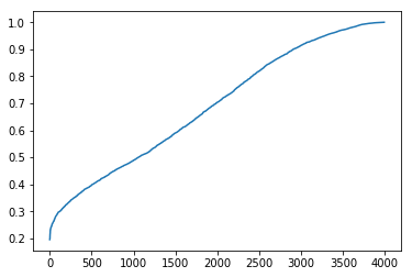
이제 Active learning을 사용하여 동일한 10%의 데이터 (400 개 샘플)에 레이블을 지정합니다. 이를 위해, 우리는 10개의 샘플 중 하나의 배치를 취하여 매우 원시적인 모델(primitive model)을 훈련시킵니다. 그런 다음이 모델을 통해 나머지 데이터 (3990 샘플)를 전달하고 최대 softmax 출력을 평가합니다. 선택한 클래스가 정답일 확률을 보여줍니다 (즉, 신경망의 신뢰도: the confidence of neural network). 정렬 후, 신뢰 분포가 20 %에서 100 %로 다양하다는 것을 플롯에서 볼 수 있습니다. LESS CONFIDENT 샘플에서 라벨을 지정할 다음 배치를 선택하는 것이 좋습니다.
# do the same in a loop for 400 samples
for i  in range(39):
    label_manually(10)
    fit()

    res = sess.run(y_sm, feed_dict={x:x_unlabeled})
    pmax = np.amax(res, axis=1)
    pidx = np.argsort(pmax)
    x_unlabeled = x_unlabeled[pidx]
    y_unlabeled = y_unlabeled[pidx]

'''
Labels: 20 	Accuracy: 0.4975
Labels: 30 	Accuracy: 0.535
Labels: 40 	Accuracy: 0.5475
Labels: 50 	Accuracy: 0.59
Labels: 60 	Accuracy: 0.64
Labels: 70 	Accuracy: 0.6475
Labels: 80 	Accuracy: 0.6925
Labels: 90 	Accuracy: 0.6975

...

Labels: 350 	Accuracy: 0.865
Labels: 360 	Accuracy: 0.8775
Labels: 370 	Accuracy: 0.8825
Labels: 380 	Accuracy: 0.8825
Labels: 390 	Accuracy: 0.885
Labels: 400 	Accuracy: 0.8975
'''
10개 샘플의 40개 배치에 대해 이러한 절차를 실행하면 결과 정확도가 거의 90%임을 알 수 있습니다. 이는 무작위로 레이블이 지정된 데이터의 경우 달성 한 83.75 %보다 훨씬 큽니다.
나머지 라벨링 되어있지 않은 데이터로 할 일
원문: What to do with the rest of the unlabeled data
# pass rest unlabeled data through the model and try to autolabel
res = sess.run(y_sm, feed_dict={x:x_unlabeled})
y_autolabeled = res.argmax(axis=1)
x_labeled = np.concatenate([x_labeled, x_unlabeled])
y_labeled = np.concatenate([y_labeled, y_autolabeled])
# train on 400 labeled by active learning and 3600 stochasticly autolabeled data
fit()

# 출력 값
# Labels: 4000	Accuracy: 0.8975
고전적인 방법은 기존 모델을 통해 나머지 데이터 세트를 실행하고 데이터에 자동으로 레이블을 지정하는 것입니다. 그런 다음 해당 데이터 세트를 훈련 과정에 넣는 것은 모델을 더 잘 조정할 수 있습니다. 위의 경우에는 더 나은 결과를 얻지 못했습니다.
My approach is to do the same but, as in the active learning, taking in consideration the confidence (이 부분을 이해하지 못했습니다,,)
# pass rest of unlabeled (3600) data trough the model for automatic labeling and show most confident samples
res = sess.run(y_sm, feed_dict={x:x_unlabeled})
y_autolabeled = res.argmax(axis=1)
pmax = np.amax(res, axis=1)
pidx = np.argsort(pmax)
# sort by confidency
x_unlabeled = x_unlabeled[pidx]
y_autolabeled = y_autolabeled[pidx]
plt.plot(pmax[pidx])
# automatically label 10 most confident sample and train for it
x_labeled = np.concatenate([x_labeled, x_unlabeled[-10:]])
y_labeled = np.concatenate([y_labeled, y_autolabeled[-10:]])
x_unlabeled = x_unlabeled[:-10]
fit()
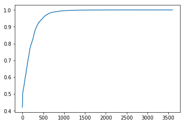
모델 평가를 통해 나머지 레이블이없는 데이터를 실행합니다. 우리는 여기서 나머지 샘플에 대한 신뢰도가 여전히 다르다는 것을 알 수 있습니다. 따라서 10개의 MOST CONFIDENT 샘플을 일괄적으로 뽑아서 모델을 교육하는 것이 좋을것 같습니다.
# run rest of unlabelled samples starting from most confident
for i in range(359):
    res = sess.run(y_sm, feed_dict={x:x_unlabeled})
    y_autolabeled = res.argmax(axis=1)
    pmax = np.amax(res, axis=1)
    pidx = np.argsort(pmax)
    x_unlabeled = x_unlabeled[pidx]
    y_autolabeled = y_autolabeled[pidx]
    x_labeled = np.concatenate([x_labeled, x_unlabeled[-10:]])
    y_labeled = np.concatenate([y_labeled, y_autolabeled[-10:]])
    x_unlabeled = x_unlabeled[:-10]
    fit()

# 출력 값
'''
Labels: 420 	Accuracy: 0.8975
Labels: 430 	Accuracy: 0.8975
Labels: 440 	Accuracy: 0.8975
Labels: 450 	Accuracy: 0.8975
Labels: 460 	Accuracy: 0.8975
Labels: 470 	Accuracy: 0.8975
Labels: 480 	Accuracy: 0.8975
Labels: 490 	Accuracy: 0.8975
Labels: 500 	Accuracy: 0.8975
Labels: 510 	Accuracy: 0.8975
Labels: 520 	Accuracy: 0.8975

...

Labels: 3850 	Accuracy: 0.9
Labels: 3860 	Accuracy: 0.9
Labels: 3870 	Accuracy: 0.9
Labels: 3880 	Accuracy: 0.905
Labels: 3890 	Accuracy: 0.905
Labels: 3900 	Accuracy: 0.905
Labels: 3910 	Accuracy: 0.905
Labels: 3920 	Accuracy: 0.905
Labels: 3930 	Accuracy: 0.905
Labels: 3940 	Accuracy: 0.905
Labels: 3950 	Accuracy: 0.905
Labels: 3960 	Accuracy: 0.905
Labels: 3970 	Accuracy: 0.905
Labels: 3980 	Accuracy: 0.905
Labels: 3990 	Accuracy: 0.905
Labels: 4000 	Accuracy: 0.905
'''
이 과정을 통해 0.8%의 정확도 향상을 얻었습니다.
결과
Experiment Accuracy
4000 샘플 92.25%
400 랜덤 샘플 83.75%
400 active learned 샘플 89.75%
+ auto-labeling 90.50%
결론
물론 이 접근방식은 연산 자원의 과도한 사용과 초기 모델 평가와 혼합된 데이터 라벨에 특별한 절차가 필요하다는 사실과 같은 단점을 가지고 있다. 또한 테스트를 위한 데이터에도 라벨을 붙여야 한다. 그러나 라벨의 비용이 높은 경우(특히 NLP, CV 프로젝트의 경우) 이 방법은 상당한 양의 자원을 절약하고 더 나은 프로젝트 결과를 가져올 수 있다.’